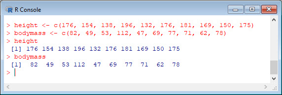
Quick start with R: Scatterplot with regression line (Part 26)

Today let’s re-create two variables and see how to plot them and include a regression line. We take height to be a variable that describes the heights (in cm) of ten people. Copy and paste the following code to the R command line to create this variable.
height <- c(176, 154, 138, 196, 132, 176, 181, 169, 150, 175)
Now let’s take bodymass to be a variable that describes the masses (in kg) of the same ten people. Copy and paste the following code to the R command line to create the weight variable.
bodymass <- c(82, 49, 53, 112, 47, 69, 77, 71, 62, 78)
Both variables are now stored in the R workspace. To view them, enter:
height bodymass

We can now create a simple plot of the two variables as follows:
plot(bodymass, height)

We can enhance this plot using various arguments within the plot() command. Copy and paste the following code into the R workspace:
plot(bodymass, height, pch = 16, cex = 1.3, col = "blue", main = "HEIGHT PLOTTED AGAINST BODY MASS", xlab = "BODY MASS (kg)", ylab = "HEIGHT (cm)")

In the above code, the syntax pch = 16 creates solid dots, while cex = 1.3 creates dots that are 1.3 times bigger than the default (where cex = 1). More about these commands later.
Now let’s perform a linear regression using lm() on the two variables by adding the following text at the command line:
lm(height ~ bodymass)

We see that the intercept is 98.0054 and the slope is 0.9528. By the way – lm stands for “linear model”.
Finally, we can add a best fit line (regression line) to our plot by adding the following text at the command line:
abline(98.0054, 0.9528)
Another line of syntax that will plot the regression line is:
abline(lm(height ~ bodymass))

None of this was so difficult! In our next blog we will look again at regression.
David

Annex: R codes used

[code lang="r"] 
# Create the height variable. 
height <- c(176, 154, 138, 196, 132, 176, 181, 169, 150, 175)

# Create the weight variable. 
bodymass <- c(82, 49, 53, 112, 47, 69, 77, 71, 62, 78)

# View both variables. 
height 
bodymass

# Create a scatterplot of height against bodymass variable. 
plot(bodymass, height)

# Create more complete scatterplot of height against bodymass variable. 
plot(bodymass, height, pch = 16, cex = 1.3, col = "blue", main = "HEIGHT PLOTTED AGAINST BODY MASS", xlab = "BODY MASS (kg)", ylab = "HEIGHT (cm)")

# Perform a linear regression on the two variables. 
lm(height ~ bodymass)

# Add a best fit line (regression line) to the plot. 
abline(98.0054, 0.9528)

# Alternatively we can plot the regression line using the following syntax: 
abline(lm(height ~ bodymass)) 
[/code]