Last time we created two variables and used the lm() command to perform a least squares regression on them, and diagnosing our regression using the plot() command. Here are the data again.
height = c(176, 154, 138, 196, 132, 176, 181, 169, 150, 175)<br />
bodymass = c(82, 49, 53, 112, 47, 69, 77, 71, 62, 78)
Just as we did last time, we perform the regression using lm(). This time we store it as an object M. Indeed – R allows you to do that!
M <- lm(height ~ bodymass)
Now we use the summary() command to obtain useful information about our regression:
summary(M)

Our model p-value is very significant (approximately 0.0004) and we have very good explanatory power (over 81% of the variability in height is explained by body mass).
We saw in the previous blog that points 2, 4, 5 and 6 have great influence on the model. Now we see how to re-fit our model while omitting one datum. Let’s omit point 6. Note the syntax we use to do so, involving the subset() command inside the lm() command and omitting the point using the syntax != which stands for “not equal to”. The syntax instructs R to fit a linear model on a subset of the data in which all points are included except the sixth point.
M2 <- lm(height ~ bodymass, subset=(1:length(height)!=6))
summary(M2)
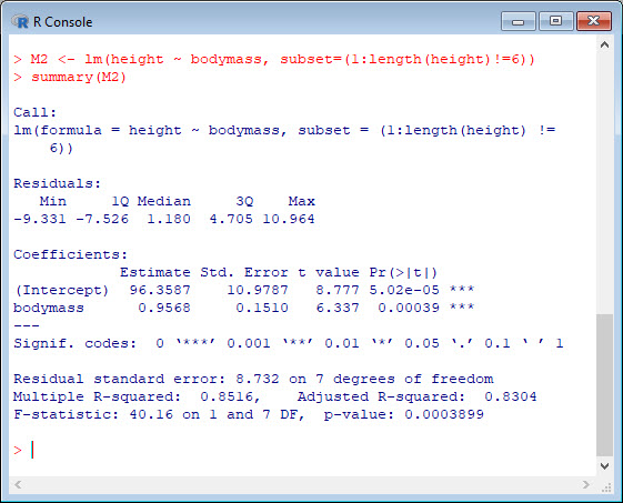
Because we have omitted one observation, we have lost one degree of freedom (from 8 to 7) but our model has greater explanatory power (i.e. the Multiple R-Squared has increased from 0.81 to 0.85). From that perspective, our model has improved, but of course, point 6 may well be a valid observation, and perhaps should be retained. Whether you omit or retain such data is a matter of judgement.
Our diagnostic plots were as follows:
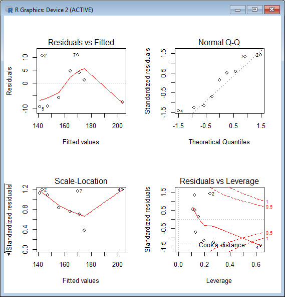
When comparing them with the diagnostic plots in previous blog we can see that there are no significant changes in these plots. In other words, omitting point 6 didn’t improve quality of the regression.
David
Annex: R codes used
# Create two variables.
height = c(176, 154, 138, 196, 132, 176, 181, 169, 150, 175)
bodymass = c(82, 49, 53, 112, 47, 69, 77, 71, 62, 78)

# Store the regression model as an object.
M <- lm(height ~ bodymass)

# Obtain useful information about regression.
summary(M)

# Store regression model as object after omitting point 6.
M2 <- lm(height ~ bodymass, subset=(1:length(height)!=6))

# Obtain useful information about new regression.
summary(M2)

# Create a plotting environment of two rows and two columns and plot the model.
par(mfrow = c(2,2))
plot(M2)

Senior Academic Manager in New Zealand Institute of Sport and Director of Sigma Statistics and Research Ltd. Author of the book: R Graph Essentials.