In Part 6, let’s look at basic plotting in R. Try entering the following three commands together (the semi-colon allows you to place several commands on the same line).

x <- seq(-4, 4, 0.2) ;  y <- 2*x^2 + 4*x - 7
plot(x, y)

This is a very basic plot, but we can do much better. Let’s build a nicer plot in several steps.

plot(x, y, pch = 16, col = "red")

The argument pch = 16 gave us solid circles, while col = "red" coloured those circles red.

Now try:

plot(x, y, pch = 16, col = "red", xlim = c(-8, 8), ylim = c(-20, 50), main = "My plot", xlab = "X variable" , ylab = "Y variable")

You can see what the main argument and the xlim and ylim arguments achieved. Now try:

plot(x, y, pch = 16, col = "red", xlim = c(-8, 8), ylim = c(-20, 50), main = "My plot", xlab = "X variable" , ylab = "Y variable")
lines(x, y)

Note that the lines() command is used after the plot() command. Now enter the following syntax.

abline(h = 0)
abline(v = 0)
abline(-10, 2)      # Draws a line of intercept -10 and slope 2.
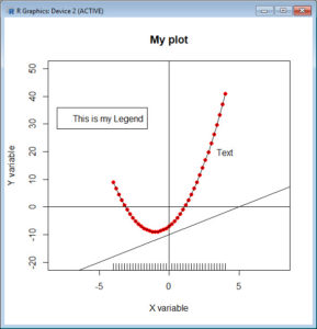
text(4, 20, "Text") # Now your text is located at the point (4, 20) on your plot.
legend(-8, 36,"This is my Legend")

Your legend is now centred on the point (-8, 36)

rug(x)

The rug() command indicates the location of points on the horizontal axis. Here is the final plot:

That wasn’t so hard! In blog 7 we will look at some more sophisticated plotting techniques in R.

Good bye for now!

David

Annex: R codes used

[code lang=”r”]
# Creating and plotting a function
x <- seq(-4, 4, 0.2); y <- 2*x^2 + 4*x – 7
plot(x, y)

# Building a nicer plot in several steps
# Version 1
plot(x, y, pch = 16, col = "red")

# Version 2
plot(x, y, pch = 16, col = "red", xlim = c(-8, 8), ylim = c(-20, 50), main = "My plot", xlab = "X variable", ylab = "Y variable")

# Version 3
plot(x, y, pch = 16, col = "red", xlim = c(-8, 8), ylim = c(-20, 50), main = "My plot", xlab = "X variable", ylab = "Y variable")
lines(x, y)

# Additional customisation
abline(h = 0)
abline(v = 0)
abline(-10, 2) # Draws a line of intercept -10 and slope 2.
text(4, 20, "Text") # Now your text is located at the point (4, 20) on your plot.
legend(-8, 36,"This is my Legend")
rug(x)
[/code]