In Part 2 we created two variables and used the lm() command to perform a least squares regression on them, treating one of them as the dependent variable and the other as the independent variable. Here they are again.
height = c(186, 165, 149, 206, 143, 187, 191, 179, 162, 185)

weight = c(89, 56, 60, 116, 51, 75, 84, 78, 67, 85)
Today we learn how to obtain useful diagnostic information about a regression model and then how to draw residuals on a plot. As before, we perform the regression.
lm(height ~ weight)

Now let’s find out more about the regression. First, let’s store the regression model as an object called first_model and then use the summary() command to learn about the regression.
first_model <- lm(height ~ weight)

summary(first_model)
Here is what R gives you.
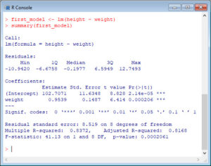
R has given you a great deal of diagnostic information about the regression. The most useful of this information are the coefficients themselves, the Adjusted R-squared, the F-statistic and the p-value for the model. I imagine that you know what these diagnostics mean.
Now let’s use R’s predict() command to create a vector of fitted values.
first_model_estimate <- predict(lm(height ~ weight))

first_model_estimate
Here are the fitted values:

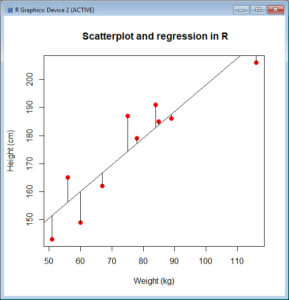
Now let’s plot the data and regression line again.
plot(weight, height, pch = 16, cex = 1.3, col = "red", main = "Scatterplot and regression in R", xlab = "Weight (kg)", ylab = "Height (cm)")

abline(102.7071, 0.9539)
We can plot the residuals using R’s for loop and a subscript k that runs from 1 to the number of data points. We know that there are 10 data points, but if we do not know the number of observations we can find it using the length() command on either the height or weight variable.
npoints <- length(weight)

npoints

Now let’s implement the loop and draw the residuals using the lines() command. Note the syntax we use to draw in the residuals.
for (k in 1: npoints) lines(c(weight[k], weight[k]), c(height[k], first_model_estimate[k]))
Here is our plot, including the residuals.
It seems none of this was so difficult! 🙂
In Part 4 we will look at more advanced aspects of regression models and see what R has to offer.
All the best for now!
David
Note: Please notice that we used in R codes both assignment operators “=” and “<-”. Thought there are some differences between these two operators, in this post they have the same effect i.e. assigning what is on the right hand side to the variable or object on the left hand side. More details about when it is appropriate to use one of these two operators are in the R manual.
Annex: R codes used
[code lang=”r”]
# Creating two variables
height = c(186, 165, 149, 206, 143, 187, 191, 179, 162, 185)
weight = c(89, 56, 60, 116, 51, 75, 84, 78, 67, 85)
# Estimating the simple linear regression
lm(height ~ weight)
# Generate an object where we store regression results
first_model <- lm(height ~ weight)
# Show regression results
summary(first_model)
# Generate estimated values for regression model
first_model_estimate <- predict(lm(height ~ weight))
# Show the estimated values of regression
first_model_estimate
# Create a scatterplot with regression line
plot(weight, height, pch = 16, cex = 1.3, col = "red", main = "Scatterplot and regression in R", xlab = "Weight (kg)", ylab = "Height (cm)")
abline(102.7071, 0.9539)
# Number of observations in the weight variable
npoints <- length(weight)
npoints
# Loop used to draw residuals on the scatterplot
for (k in 1: npoints) lines(c(weight[k], weight[k]), c(height[k], first_model_estimate[k]))
[/code]

Senior Academic Manager in New Zealand Institute of Sport and Director of Sigma Statistics and Research Ltd. Author of the book: R Graph Essentials.